
Unconstrained nonlinear programming: Nelder-Mead Simplex algorithm
In the previous two posts, I have described the basics of penalty methods (exterior and interior), and how they can be used to solve constrained nonlinear optimisation problems using unconstrained nonlinear programming algorithms. In this post, I will take a step back, and describe the simplest (yet quite powerful) heuristic algorithm for unconstrained nonlinear programming: the Nelder-Mead Simplex algorithm.
The algorithm
The algorithm tries to minimise the objective function, \(f\), by successively re-evaluating the so-called simplices in the direction where the function decreases in value [1], [2]. A simplex is a generalisation of the triangle to multi-dimensional spaces. In a 2-dimensional space, the simplex is still just a triangle. Therefore, to keep things simple, the entire post will assume minimisation in 2 dimensions.
Suppose we are given simplex with the following vertices \(\{x_0, x_1, x_2\}\), \(x_i\in\mathbb{R}^2\) for each \(i\). Let’s re-order the vertices by the increasing function value; that is, let \(\{x^L, x^M, x^H\}\) such that \(f(x^L) \le f(x^M) \le f(x^H)\). The main idea of the algorithm is to replace the point which maximises the function in the current simplex with a new, better point, \(x'\) say, in the sense that it minimises the function with respect to \(x^H\); that is, \(f(x') < f(x^H)\). This can be achieved in one of the 4 possible ways: by reflection, expansion, contraction, and shrinking.
Reflection
In the reflection step, the point for which the function achieves the highest value, \(x^H\), is potentially replaced with a point that is reflected against the edge of the simplex connecting the remaining points. That is, if you imagine the edge connecting the points \(x^L\) — \(x^M\) being a mirror, we reflect \(x^H\) against that mirror:
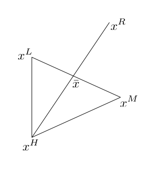
Or mathematically
\[\begin{equation} x^R = \bar{x} + \alpha(\bar{x} - x^H) \end{equation}\]where \(\alpha>0\) (and usually \(\alpha=1\)), and \(\bar{x} = \frac{x^L + x^M}{2}\) is the centroid (or the centre of gravity) of the points \(x^L\) and \(x^M\). The reasoning behind the reflection step is that since the points \(x^L\) and \(x^M\) minimise the function for the current simplex, by reflecting \(x^H\) against these two points, we should potentially move in the direction that further minimises the function; that is, \(f(x^R) \le f(x^H)\).
Expansion
If it so happens that the reflected point is better than the current minimum, i.e., if \(f(x^R) < f(x^L)\), then perhaps by moving even further in that direction, we’ll further minimise the function. This step is referred to as the expansion step:
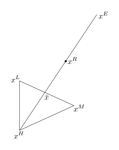
Or mathematically
\[\begin{equation} x^E = \bar{x} + \gamma(x^R - \bar{x}) \end{equation}\]where \(\gamma > 1\), and typically \(\gamma = 2\).
Contraction
If, however, the reflected point, \(x^R\) does not offer a significant improvement over \(x^H\), i.e., if \(f(x^H) \ge f(x^R) > f(x^M)\), then we need to test for points between either the reflected point and the centroid, or the highest value point and the centroid. If \(f(x^R) < f(x^H)\), then we choose the first pair; otherwise, we settle on the latter one. Having selected the appropriate pair of points, we contract the distance between the two. Suppose for the moment that we have selected \(x^R\) to contract against. Then, the contraction step looks as follows:
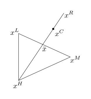
Or mathematically
\[\begin{equation} x^C = \bar{x} + \beta(x^R - \bar{x}) \end{equation}\]where \(0 < \beta < 1\), and typically \(\beta = \frac{1}{2}\).
Shrinking
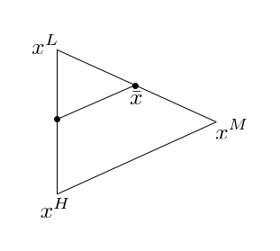
If the contraction step fails, that is, if \(f(x^C) \ge f(x^H)\), then, as the last resort, we shrink the simplex by half towards the current minimum, \(x^L\):
The algorithm revisited
Taking it all together, the algorithm proceeds as follows. For any given simplex \(\{x^L, x^M, x^H\}\), compute the reflected point, \(x^R\).
If \(f(x^R) < f(x^L)\), then compute the expanded point, \(x^E\). If \(f(x^E) < f(x^R)\), then assign \(x^H := x^E\), and start over. Otherwise, assign \(x^H := x^R\), and start over.
If \(f(x^L) \le f(x^R) \le f(x^M)\), then assign \(x^H := x^R\), and start over. Otherwise, select \(x' = \arg\min(f(x^H), f(x^R))\). Compute the contracted point, \(x^C\). If \(f(x^C) \le f(x')\), then assign \(x^H := x^C\), and start over. Otherwise, shrink the simplex, and start over.
Examples
Having described the theory, let’s look at some examples. The full source code for the examples shown in this post can be downloaded from GitHub.
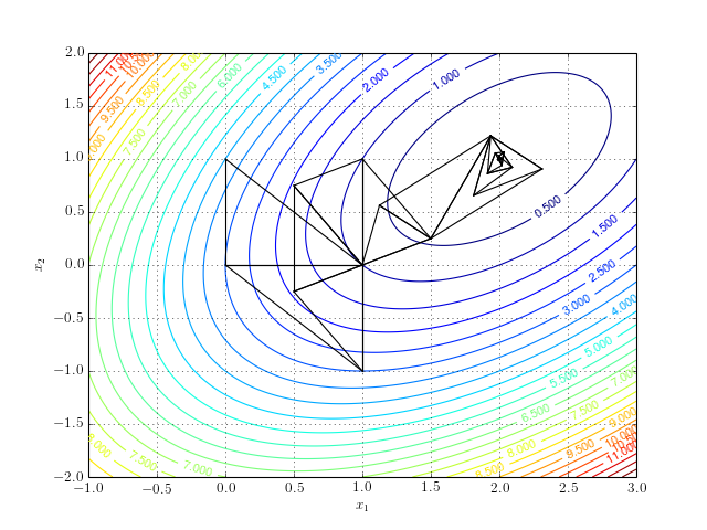
Firstly, consider minimising the function
\[\begin{equation} f(x_1, x_2) = x_1^2 + x_2^2 - 3x_1 - x_1x_2 + 3. \end{equation}\]This function has one global minimum at a point \(x = (2, 1)\). The path of the simplex algorithm is overlaid on the contour plot of the objective function:
And a more interactive version:
Notice that the algorithm after a series of reflection, expansion, contraction, and shrinking steps converges to the minimum.
Multiple minima
It becomes quite problematic for the algorithm if the function under consideration has more than one minimum. Then, the algorithm is not guaranteed to converge to the global one. Consider an example
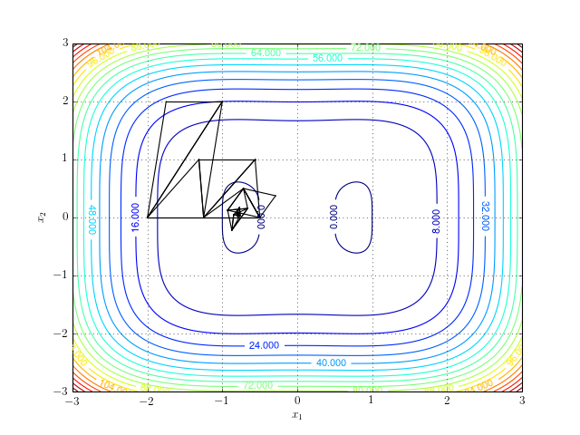
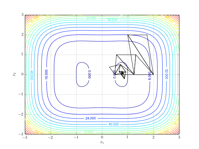
\[\begin{equation} f(x_1, x_2) = x_1^4 + x_2^4 - \frac{5}{4} x_1^2 + \frac{1}{4}. \end{equation}\]This function has two minima at points \((0.8, 0)\) and \((-0.8, 0)\). Depending on the choice of the initial simplex, the algorithm might converge to either of the two. Therefore, it is important to correctly pick the initial simplex for a given problem.
For example, starting off with the simplex \(\{(-2,0), (-1,2), (-1.75,2)\}\) produces the following result:
While, starting off at \(\{(2,0), (1,2), (1.75,2)\}\), produces:
No minimum
Finally, if the function does not have a minimum, then the algorithm will inevitably fail to converge (which is as expected). However, if you are attempting to implement your own version of the Simplex algorithm, it is important to remember about this eventuality. After all, in real world, it is sometimes almost impossible to determine whether the problem we are trying to optimise has an optimum value.
Consider an example
\[\begin{equation} f(x_1, x_2) = x_1x_2. \end{equation}\]The function does not have a minimum (nor a maximum). However, it does have a stationary point at \((0,0)\). If we run the simplex algorithm in the search of a minimum, it will never converge. The following contour plot shows the search path for 8 iterations of the algorithm:
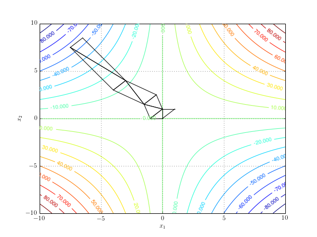
And a more interactive version:
References
[1] Avriel, M., “Nonlinear Programming: Analysis and Methods”, chapter 9, Dover Publications, 2003.
[2] Mathews, J. H., and Fink, K. K., “Numerical Methods Using Matlab, 4th edition”, chapter 8, Prentice-Hall Inc., 2004. Excerpt on Nelder-Mead Simplex algorithm available here.